Conditional formatting in Tables and Matrixes
Power BI Desktop and Power BI Service Conditional Formatting for Tables and Matrices
Conditional formatting in Power BI enables you to enhance your tables and matrices by specifying customized cell colors, including color gradients, based on field values. You can also represent cell values with data bars, KPI icons, or as active web links. This feature is applicable to both Power BI Desktop and Power BI Service.
How to Apply Conditional Formatting:
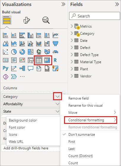
Select Visualization: Begin by selecting a Table or Matrix visualization in Power BI Desktop or the Power BI service.
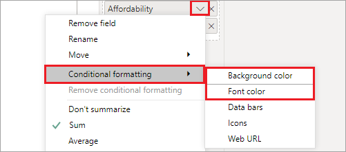
Access Conditional Formatting: In the Visualizations pane, right-click or select the down-arrow next to the field in the Values well that you want to format. Choose
“Conditional formatting,” and then select the desired formatting type.
Note: Conditional formatting overrides any custom background or font colors applied to the conditionally formatted cell.
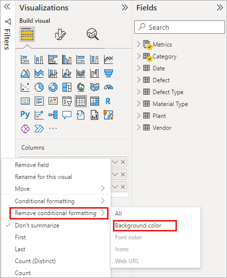
Remove Conditional Formatting: To remove conditional formatting, select “Remove conditional formatting” from the field’s drop-down menu, and then choose the formatting type to remove.
Conditional Formatting Options:
1. Format Background or Font Color
To format cell background or font color, select Conditional formatting for a field and choose “Background color” or “Font color” from the drop-down menu.
2. Color by Color Scale
This option allows you to format cell background or font color using a color scale. Specify the field to base formatting on, summarization type, and color scheme.
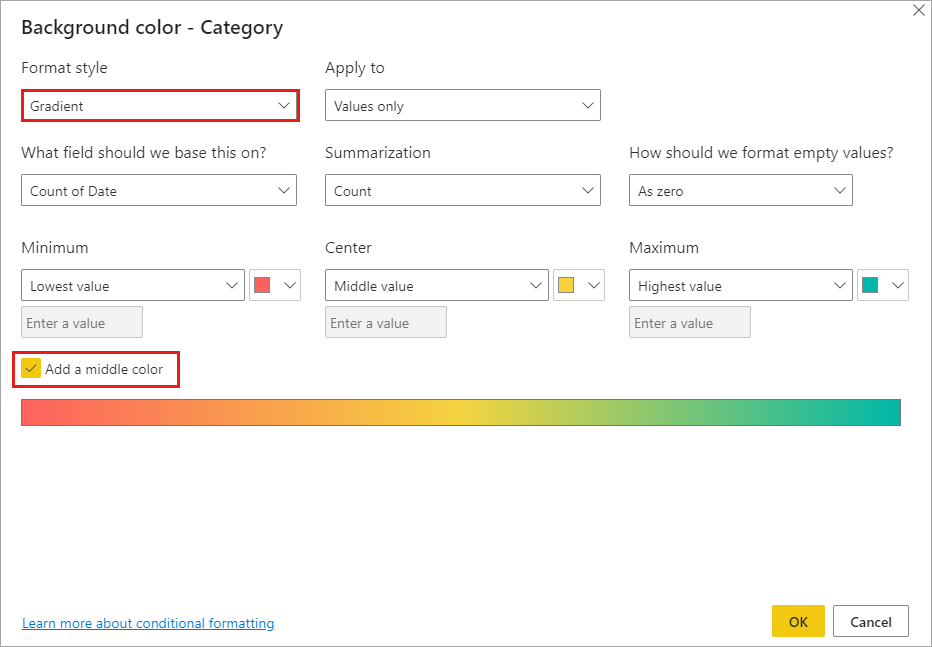
- In the Format style field, choose Gradient in the Background color or Font color dialog box.
- Select the field for formatting based on, either the current field or any field with numerical or color data.
- Specify the aggregation type under Summarization.
- Choose a formatting option for blank values under Default formatting.
- Decide whether to use the lowest and highest field values or custom values for the color scheme under Minimum and Maximum.
- Select colors for the minimum and maximum values.
Optionally, add a middle color by checking the box and specify a Center value and color.
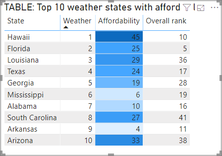
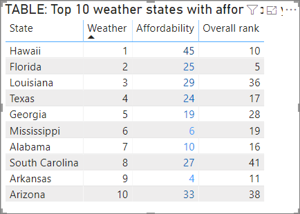
An example table with color scale background formatting on the Affordability column looks like this:
The example table with color scale font formatting on the Affordability column looks like this:
3. Color by Rules:
Format cell background or font color based on defined rules. Set value ranges and assign colors to each range.
- In the Format style field of the Background color or Font color dialog box, choose Rules.
- Determine the field for formatting by referring to “What field should we base this on?” and specify the aggregation type with “Summarization.”
Under the Rules option, do the following:
- Define one or more value ranges.
- Assign a color to each value range.
- Each value range consists of an If value condition, an and value condition, and a color.
- Cell backgrounds or fonts within each value range will be colored according to the specified color.
For instance, consider the following example with three rules:
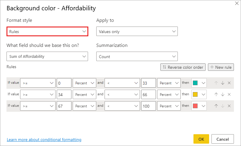
Choosing “Percent” in this dropdown means you’re establishing rule boundaries as a percentage of the total range of values, spanning from the minimum to the maximum. For instance, if the lowest data point is 100 and the highest is 400, using the mentioned rules would result in points below 200 being colored green, those between 200 and 300 as yellow, and any value exceeding 300 as red.
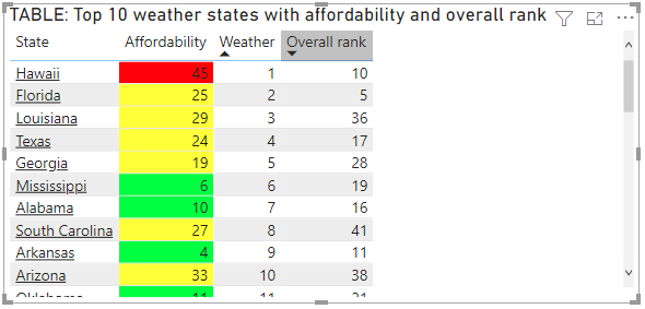
Here’s an example table showcasing background color formatting based on “Percent” in the Affordability column:
4. Color by Rules for Percentages
If the field you’re using for formatting contains percentages, express the numbers in the rules as decimals, which represent the actual values. For instance, use “.25” instead of “25”. Additionally, choose “Number” instead of “Percent” for the number format. For example, if you set a rule as “If the value is greater than or equal to 0 Number and less than .25 Number,” it will identify values less than 25%.
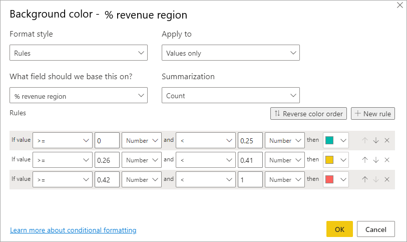
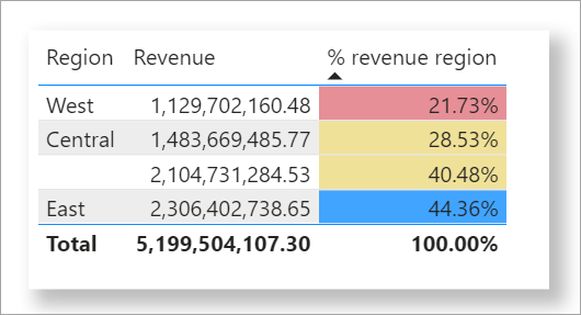
In this sample table with background color formatting rules applied to the % revenue region column:
- Values from 0 to 25% are colored red.
- Values between 26% and 41% are colored yellow.
- Values at 42% or higher are colored blue.
5. Color by Color Values
You can format a column’s background or font color using conditional formatting based on:
- Hexadecimal values: Use 3, 6, or 8-digit hex codes, e.g., #3E4AFF (ensure you include the # symbol at the start).
- RGB or RGBA values: Specify color with RGB or RGBA, like RGBA(234, 234, 234, 0.5).
- HSL or HSLA values: Utilize HSL or HSLA values, such as HSLA(123, 75%, 75%, 0.5).
- Color names: Apply color names like Green, SkyBlue, or PeachPuff.
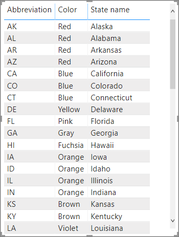
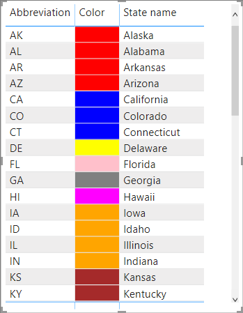
For example, the table below associates a color name with each state:
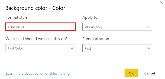
To format the Color column based on its field values, select Conditional formatting for the Color field, and then select Background color or Font color.
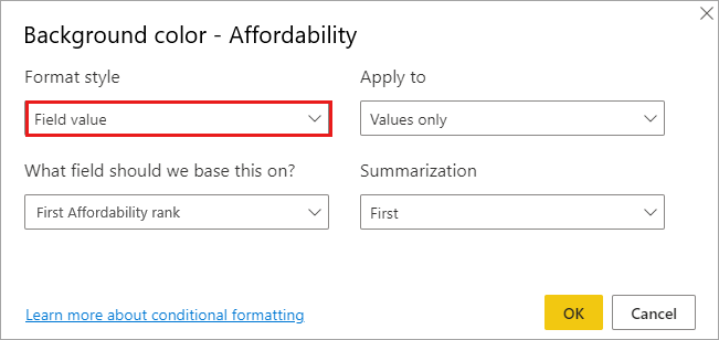
In the Background color or Font color dialog box, select Field value from the Format style drop-down field.
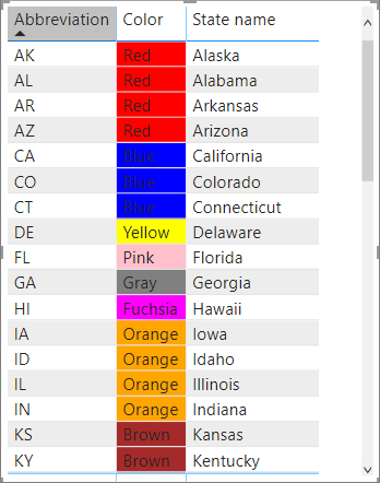
An example table with color field value-based Background color formatting on the Color field looks like this:
If you also use Field value to format the column’s Font color, the result is a solid color in the Color column:
6. Color Based on a Calculation
You can create a calculation that outputs different values based on business logic conditions you select. Creating a formula is usually faster than creating multiple rules in the conditional formatting dialog.
For example, the following formula applies hex color values to a new Affordability rank column, based on existing Affordability column values:
To apply the colors, select Background color or Font color conditional formatting for the Affordability column, and base the formatting on the Field value of the Affordability rank column.
The example table with Affordability background color based on calculated Affordability rank looks like this:
7. Add Data Bars
- Click on Conditional formatting for the Affordability field.
- From the drop-down menu, choose Data bars.
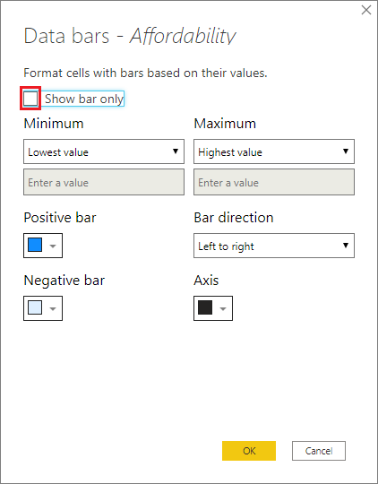
In the Data bars dialog:
- By default, the “Show bar only” option is unchecked, allowing both bars and actual values in the table cells. To display only the data bars, check the “Show bar only” box.
- You can define Minimum and Maximum values, choose data bar colors and direction, and set the axis color.
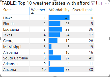
With data bars applied to the Affordability column, the example table looks like this:
8. Add Icons
To display icons based on cell values:
- Choose Conditional formatting for the field.
- From the drop-down menu, select Icons.
In the Icons dialog:
- Under Format style, opt for either Rules or Field value.
To format using rules:
- Select a field for the basis (“What field should we base this on?”).
- Specify the Summarization method, Icon layout, Icon alignment, and Icon Style.
- Define one or more Rules. For each rule, set conditions with “If value” and “and value” conditions and select an icon.
To format based on field values:
- Choose a field for the basis (“What field should we base this on?”).
- Set the Summarization method, Icon layout, and Icon alignment.
- For example, the following illustration demonstrates adding icons based on three rules:
Select OK. With icons applied to the Affordability column by rules, the example table looks like this:
9. Format as Web URLs
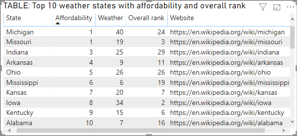
If you have a column or measure that contains website URLs, you can use conditional formatting to apply those URLs to fields as active links. For example, the following table has a Website column with website URLs for each state:
To make each state name a clickable link to its website:
- Click on Conditional formatting for the State field.
- Choose Web URL.
In the Web URL dialog:
Under “What field should we base this on?”, select Website, and then click OK.
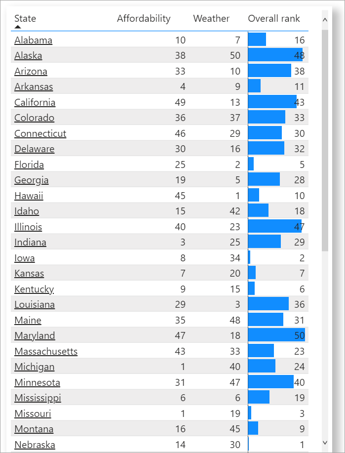
With Web URL formatting enabled for the State field, each state name now functions as a live link to its respective website. In the example table below, the State column has Web URL formatting, while the Overall rank column has conditional Data bars applied.
Totals and Subtotals
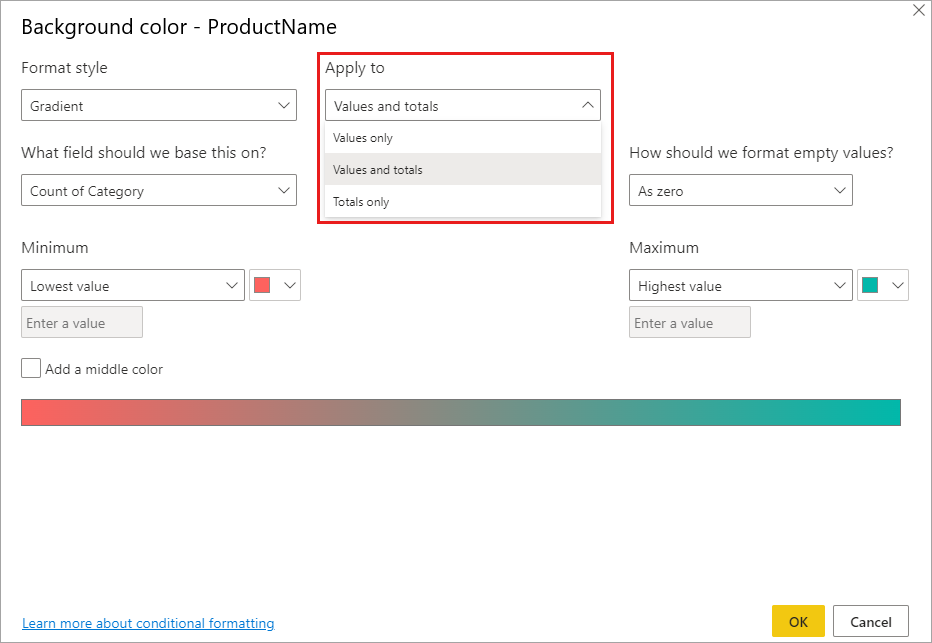
You can apply conditional formatting rules to totals and subtotals, for both table and matrix visuals.
You apply the conditional formatting rules by using the Apply to drop-down in conditional formatting, as shown in the following image.
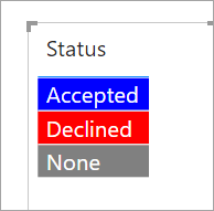
Color-Code Based on Text
In contrast to Excel, you can’t directly assign specific colors to text values like “Accepted”=blue, “Declined”=red, “None”=grey. Instead, you need to create measures that associate these values with colors and then apply formatting based on these measures.
For instance, you can create a measure called StatusColor using SWITCH function:
Afterward, in the Background color dialog box, you can format the Status field based on the values provided by the StatusColor measure.
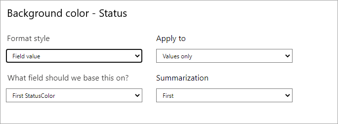
In the resulting table, the formatting is based on the value in the StatusColor field, which in turn is based on the text in the Status field.
Considerations and Limitations
- Conditional formatting may require aggregation or measures to be applied to values.
- Considerations related to NaN values and printing reports with conditional formatting are mentioned.
Conditional formatting in Power BI is a powerful tool that allows you to make your tables and matrices visually informative and appealing, highlighting important data based on specific conditions or criteria.